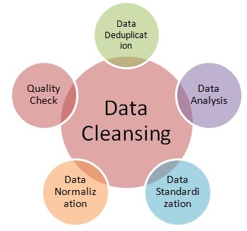
This notebook deals with the data cleaning, and walks through the steps of data cleaning in a good quality practice.
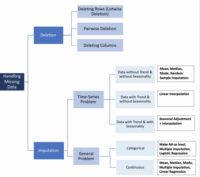
Part (1) of the (5) in Data Cleaning process! We are going to be looking at how to deal with missing values.
*In statistics, missing data, or missing values, occur when no data value is stored for the variable in an observation. Missing data are a common occurrence and can have a significant effect on the conclusions that can be drawn from the data. Missing data can occur because of nonresponse: no information is provided for one or more items or a whole unit ("subject"). Some items are more likely to generate a nonresponse than others: items about private subjects such as income. Attrition is a type of missingness that can occur in longitudinal studies—for instance, studying development where a measurement is repeated after a certain period of time. Missingness occurs when participants drop out before the test ends, and one or more measurements are missing.
In part (1) we will:
The first thing we will need to do is load in the libraries and datasets we will be using. We will be using a dataset of events that occured in American Football games for demonstration.
Important! Make sure we run this cell ourself or the rest of our code won't work!
# modules we will use
import pandas as pd
import numpy as np
import warnings

warnings.filterwarnings("ignore")

# read in all our data
nfl_data = pd.read_csv("NFL Play by Play 2009-2017 (v4).csv")

# set seed for reproducibility
np.random.seed(0)
The first thing we do when we get a new dataset is take a look at some of it. This lets us see that it all read incorrectly and get an idea of what is going on with the data. In this case, we are looking to see if we see any missing values, which will be reprsented with NaN or None.
# looking at a few rows of the nfl_data file. We can see a few missing data already!
nfl_data.sample(5)
| Date | GameID | Drive | qtr | down | time | TimeUnder | TimeSecs | PlayTimeDiff | SideofField | ... | yacEPA | Home_WP_pre | Away_WP_pre | Home_WP_post | Away_WP_post | Win_Prob | WPA | airWPA | yacWPA | Season | |
|---|---|---|---|---|---|---|---|---|---|---|---|---|---|---|---|---|---|---|---|---|---|
| 244485 | 2014-10-26 | 2014102607 | 18 | 3 | 1.0 | 00:39 | 1 | 939.0 | 12.0 | TB | ... | 1.240299 | 0.225647 | 0.774353 | 0.245582 | 0.754418 | 0.225647 | 0.019935 | -0.018156 | 0.038091 | 2014 |
| 115340 | 2011-11-20 | 2011112000 | 22 | 4 | 1.0 | 06:47 | 7 | 407.0 | 44.0 | OAK | ... | NaN | 0.056036 | 0.943964 | 0.042963 | 0.957037 | 0.943964 | 0.013073 | NaN | NaN | 2011 |
| 68357 | 2010-11-14 | 2010111401 | 8 | 2 | NaN | 00:23 | 1 | 1823.0 | 0.0 | CLE | ... | NaN | 0.365307 | 0.634693 | 0.384697 | 0.615303 | 0.634693 | -0.019390 | NaN | NaN | 2010 |
| 368377 | 2017-09-24 | 2017092405 | 24 | 4 | 1.0 | 08:48 | 9 | 528.0 | 8.0 | CLE | ... | 1.075660 | 0.935995 | 0.064005 | 0.921231 | 0.078769 | 0.064005 | 0.014764 | 0.003866 | 0.010899 | 2017 |
| 384684 | 2017-11-05 | 2017110505 | 11 | 2 | 1.0 | 09:15 | 10 | 2355.0 | 0.0 | DEN | ... | NaN | 0.928474 | 0.071526 | 0.934641 | 0.065359 | 0.071526 | -0.006166 | NaN | NaN | 2017 |
5 rows × 102 columns
We do have some missing values. We will see how many we have in each column.
# get the number of missing data points per column
missing_values_count = nfl_data.isnull().sum()

# look at the # of missing points in the first ten columns
missing_values_count[0:10]
Date                0
GameID              0
Drive               0
qtr                 0
down            61154
time              224
TimeUnder           0
TimeSecs          224
PlayTimeDiff      444
SideofField       528
dtype: int64
That seems like a lot! It might be helpful to see what percentage of the values in our dataset were missing to give us a better sense of the scale of this problem:
# how many total missing values do we have?
total_cells = np.product(nfl_data.shape)
total_missing = missing_values_count.sum()

# percent of data that is missing
(total_missing/total_cells) * 100
24.87214126835169
Quarter of the cells in this dataset are empty! In the next step, we are going to take a closer look at some of the columns with missing values and try to figure out what might be going on with them.
This is the point at which we get into the part of data science that we like to call "data intution", by which we mean "really looking at our data and trying to figure out why it is the way it is and how that will affect our analysis". It can be a frustrating part of data science, especially if we are newer to the field and do not have a lot of experience. For dealing with missing values, we will need to use our intution to figure out why the value is missing. One of the most important question we can ask ourself to help figure this out is this:
Is this value missing becuase it was not recorded or becuase it dose not exist?
If a value is missing becuase it does not exist (like the height of the oldest child of someone who does not have any children) then it does not make sense to try and guess what it might be. These values we probalby do want to keep as NaN. On the other hand, if a value is missing becuase it was not recorded, then we can try to guess what it might have been based on the other values in that column and row. (This is called "imputation" and we will learn how to do it!
We will work through an example. Looking at the number of missing values in the nfl_data dataframe, we notice that the column TimesSec has a lot of missing values in it:
# look at the # of missing points in the first ten columns
missing_values_count[0:10]
Date                0
GameID              0
Drive               0
qtr                 0
down            61154
time              224
TimeUnder           0
TimeSecs          224
PlayTimeDiff      444
SideofField       528
dtype: int64
By looking at the business documentation, we will assume this column has information on the number of seconds left in the game when the play was made. This means that these values are probably missing because they were not recorded, rather than because they do not exist. So, it would make sense for us to try and guess what they should be rather than just leaving them as NA's.
On the other hand, there are other fields, like PenalizedTeam that also have lot of missing fields. In this case, though, the field is missing because if there was no penalty then it does not make sense to say which team was penalized. For this column, it would make more sense to either leave it empty or to add a third value like "neither" and use that to replace the NA's.
Always: Read over the dataset documentation if we have not already! If we are working with a dataset that we have gotten from another department, we can also try reaching out to them to get more information.
If we are doing very careful data analysis, this is the point at which we would look at each column individually to figure out the best strategy for filling those missing values. For the rest of this notebook, we will cover some techniques that can help us with missing values but will probably also end up removing some useful information or adding some noise to our data.
If we are in a hurry don not have a reason to figure out why our values are missing, one option we have is to just remove any rows or columns that contain missing values. (Note: We do not generally recommend this approch for important projects! It is usually worth it to take the time to go through our data and look at all the columns with missing values one-by-one to really get to know our dataset.)
If we are sure we want to drop rows with missing values, pandas does have a handy function, dropna() to help us do this. We will try it out on our NFL dataset!
# remove all the rows that contain a missing value
nfl_data.dropna()
| Date | GameID | Drive | qtr | down | time | TimeUnder | TimeSecs | PlayTimeDiff | SideofField | ... | yacEPA | Home_WP_pre | Away_WP_pre | Home_WP_post | Away_WP_post | Win_Prob | WPA | airWPA | yacWPA | Season |
|---|
0 rows × 102 columns
Looks like that is removed all our data! This is because every row in our dataset had at least one missing value. We might have better output removing all the columns that have at least one missing value instead.
# remove all columns with at least one missing value
columns_with_na_dropped = nfl_data.dropna(axis=1)
columns_with_na_dropped.head()
| Date | GameID | Drive | qtr | TimeUnder | ydstogo | ydsnet | PlayAttempted | Yards.Gained | sp | ... | Timeout_Indicator | Timeout_Team | posteam_timeouts_pre | HomeTimeouts_Remaining_Pre | AwayTimeouts_Remaining_Pre | HomeTimeouts_Remaining_Post | AwayTimeouts_Remaining_Post | ExPoint_Prob | TwoPoint_Prob | Season | |
|---|---|---|---|---|---|---|---|---|---|---|---|---|---|---|---|---|---|---|---|---|---|
| 0 | 2009-09-10 | 2009091000 | 1 | 1 | 15 | 0 | 0 | 1 | 39 | 0 | ... | 0 | None | 3 | 3 | 3 | 3 | 3 | 0.0 | 0.0 | 2009 |
| 1 | 2009-09-10 | 2009091000 | 1 | 1 | 15 | 10 | 5 | 1 | 5 | 0 | ... | 0 | None | 3 | 3 | 3 | 3 | 3 | 0.0 | 0.0 | 2009 |
| 2 | 2009-09-10 | 2009091000 | 1 | 1 | 15 | 5 | 2 | 1 | -3 | 0 | ... | 0 | None | 3 | 3 | 3 | 3 | 3 | 0.0 | 0.0 | 2009 |
| 3 | 2009-09-10 | 2009091000 | 1 | 1 | 14 | 8 | 2 | 1 | 0 | 0 | ... | 0 | None | 3 | 3 | 3 | 3 | 3 | 0.0 | 0.0 | 2009 |
| 4 | 2009-09-10 | 2009091000 | 1 | 1 | 14 | 8 | 2 | 1 | 0 | 0 | ... | 0 | None | 3 | 3 | 3 | 3 | 3 | 0.0 | 0.0 | 2009 |
5 rows × 41 columns
# just how much data did we lose?
print("Columns in original dataset: %d \n" % nfl_data.shape[1])
print("Columns with na's dropped: %d" % columns_with_na_dropped.shape[1])
Columns in original dataset: 102

Columns with na's dropped: 41
We have lost quite a bit of data, but at this point we have successfully removed all the NaN's from our data.
Another option is to try and fill in the missing values. For this next bit, We getting a small sub-section of the NFL data so that it will print well.
# get a small subset of the NFL dataset
subset_nfl_data = nfl_data.loc[:, 'EPA':'Season'].head()
subset_nfl_data
| EPA | airEPA | yacEPA | Home_WP_pre | Away_WP_pre | Home_WP_post | Away_WP_post | Win_Prob | WPA | airWPA | yacWPA | Season | |
|---|---|---|---|---|---|---|---|---|---|---|---|---|
| 0 | 2.014474 | NaN | NaN | 0.485675 | 0.514325 | 0.546433 | 0.453567 | 0.485675 | 0.060758 | NaN | NaN | 2009 |
| 1 | 0.077907 | -1.068169 | 1.146076 | 0.546433 | 0.453567 | 0.551088 | 0.448912 | 0.546433 | 0.004655 | -0.032244 | 0.036899 | 2009 |
| 2 | -1.402760 | NaN | NaN | 0.551088 | 0.448912 | 0.510793 | 0.489207 | 0.551088 | -0.040295 | NaN | NaN | 2009 |
| 3 | -1.712583 | 3.318841 | -5.031425 | 0.510793 | 0.489207 | 0.461217 | 0.538783 | 0.510793 | -0.049576 | 0.106663 | -0.156239 | 2009 |
| 4 | 2.097796 | NaN | NaN | 0.461217 | 0.538783 | 0.558929 | 0.441071 | 0.461217 | 0.097712 | NaN | NaN | 2009 |
We can use the Panda's fillna() function to fill in missing values in a dataframe for us. One option we have is to specify what we want the NaN values to be replaced with. We would like to replace all the NaN values with 0.
# replace all NA's with 0
subset_nfl_data.fillna(0)
| EPA | airEPA | yacEPA | Home_WP_pre | Away_WP_pre | Home_WP_post | Away_WP_post | Win_Prob | WPA | airWPA | yacWPA | Season | |
|---|---|---|---|---|---|---|---|---|---|---|---|---|
| 0 | 2.014474 | 0.000000 | 0.000000 | 0.485675 | 0.514325 | 0.546433 | 0.453567 | 0.485675 | 0.060758 | 0.000000 | 0.000000 | 2009 |
| 1 | 0.077907 | -1.068169 | 1.146076 | 0.546433 | 0.453567 | 0.551088 | 0.448912 | 0.546433 | 0.004655 | -0.032244 | 0.036899 | 2009 |
| 2 | -1.402760 | 0.000000 | 0.000000 | 0.551088 | 0.448912 | 0.510793 | 0.489207 | 0.551088 | -0.040295 | 0.000000 | 0.000000 | 2009 |
| 3 | -1.712583 | 3.318841 | -5.031425 | 0.510793 | 0.489207 | 0.461217 | 0.538783 | 0.510793 | -0.049576 | 0.106663 | -0.156239 | 2009 |
| 4 | 2.097796 | 0.000000 | 0.000000 | 0.461217 | 0.538783 | 0.558929 | 0.441071 | 0.461217 | 0.097712 | 0.000000 | 0.000000 | 2009 |
We could replace missing values with whatever value comes directly after it in the same column. (This makes a lot of sense for datasets where the observations have some sort of logical order to them.)
# replace all NA's the value that comes directly after it in the same column,
# then replace all the reamining na's with 0
subset_nfl_data.fillna(method = 'bfill', axis=0).fillna(0)
| EPA | airEPA | yacEPA | Home_WP_pre | Away_WP_pre | Home_WP_post | Away_WP_post | Win_Prob | WPA | airWPA | yacWPA | Season | |
|---|---|---|---|---|---|---|---|---|---|---|---|---|
| 0 | 2.014474 | -1.068169 | 1.146076 | 0.485675 | 0.514325 | 0.546433 | 0.453567 | 0.485675 | 0.060758 | -0.032244 | 0.036899 | 2009 |
| 1 | 0.077907 | -1.068169 | 1.146076 | 0.546433 | 0.453567 | 0.551088 | 0.448912 | 0.546433 | 0.004655 | -0.032244 | 0.036899 | 2009 |
| 2 | -1.402760 | 3.318841 | -5.031425 | 0.551088 | 0.448912 | 0.510793 | 0.489207 | 0.551088 | -0.040295 | 0.106663 | -0.156239 | 2009 |
| 3 | -1.712583 | 3.318841 | -5.031425 | 0.510793 | 0.489207 | 0.461217 | 0.538783 | 0.510793 | -0.049576 | 0.106663 | -0.156239 | 2009 |
| 4 | 2.097796 | 0.000000 | 0.000000 | 0.461217 | 0.538783 | 0.558929 | 0.441071 | 0.461217 | 0.097712 | 0.000000 | 0.000000 | 2009 |
Filling in missing values is also known as "imputation"
Part (2) of the (5) in Data Cleaning process! We are going to be looking at how to deal withscale and normalize data (and what the difference is between the two!).
Feature scaling is a method used to normalize the range of independent variables or features of data. Data processing is also known as data normalization and is generally performed during the data preprocessing step.
In part (2) we will:
The first thing we will need to do is load in the libraries and datasets we will be using.
Important! Make sure we run this cell ourself or the rest of our code won't work!
# modules we will use
import pandas as pd
import numpy as np

# for Box-Cox Transformation
from scipy import stats

# for min_max scaling
from mlxtend.preprocessing import minmax_scaling

# plotting modules
import seaborn as sns
import matplotlib.pyplot as plt

# read in all our data
kickstarters_2017 = pd.read_csv("ks-projects-201801.csv")

# set seed for reproducibility
np.random.seed(0)
One of the reasons that it is easy to get confused between scaling and normalization is because the terms are sometimes used interchangeably and, to make it even more confusing, they are very similar! In both cases, we are transforming the values of numeric variables so that the transformed data points have specific helpful properties. The difference is that, in scaling, we are changing the range of our data while in normalization we are changing the shape of the distribution of our data.
This means that we are transforming our data so that it fits within a specific scale, like 0-100 or 0-1. We want to scale data when we are using methods based on measures of how far apart data points, like support vector machines, or SVM or k-nearest neighbors, or KNN. With these algorithms, a change of "1" in any numeric feature is given the same importance.
For example, we might be looking at the prices of some products in both Yen and US Dollars. One US Dollar is worth about 100 Yen, but if we do not scale our prices methods like SVM or KNN will consider a difference in price of 1 Yen as important as a difference of 1 US Dollar! This clearly does not fit with our intuitions of the world. With currency, we can convert between currencies. But what about if we are looking at something like height and weight? It is not entirely clear how many pounds should equal one inch (or how many kilograms should equal one meter).
By scaling our variables, we can help compare different variables on equal footing. To help solidify what scaling looks like, we will look at a made-up example.
# generate 1000 data points randomly drawn from an exponential distribution
original_data = np.random.exponential(size = 1000)

# mix-max scale the data between 0 and 1
scaled_data = minmax_scaling(original_data, columns = [0])

# plot both together to compare
fig, ax=plt.subplots(1,2)
sns.distplot(original_data, ax=ax[0])
ax[0].set_title("Original Data")
sns.distplot(scaled_data, ax=ax[1])
ax[1].set_title("Scaled data")
Text(0.5, 1.0, 'Scaled data')

We notice that the shape of the data does not change, but that instead of ranging from 0 to 8, it now ranges from 0 to 1.
Scaling just changes the range of our data. Normalization is a more radical transformation. The point of normalization is to change our observations so that they can be described as a normal distribution.
Normal distribution: Also known as the "bell curve", this is a specific statistical distribution where a roughly equal observations fall above and below the mean, the mean and the median are the same, and there are more observations closer to the mean. The normal distribution is also known as the Gaussian distribution.
In general, we will only want to normalize our data if we are going to be using a machine learning or statistics technique that assumes our data is normally distributed. Some examples of these include t-tests, ANOVAs, linear regression, linear discriminant analysis (LDA) and Gaussian naive Bayes. (Pro tip: any method with "Gaussian" in the name probably assumes normality.)
The method were using to normalize here is called the Box-Cox Transformation. We will take a quick peek at what normalizing some data looks like:
# normalize the exponential data with boxcox
normalized_data = stats.boxcox(original_data)

# plot both together to compare
fig, ax=plt.subplots(1,2)
sns.distplot(original_data, ax=ax[0])
ax[0].set_title("Original Data")
sns.distplot(normalized_data[0], ax=ax[1])
ax[1].set_title("Normalized data")
Text(0.5, 1.0, 'Normalized data')

Notice that the shape of our data has changed. Before normalizing it was almost L-shaped. But after normalizing it looks more like the outline of a bell (hence "bell curve").
To practice scaling and normalization, we are going to be using a dataset of Kickstarter campaigns. (Kickstarter is a website where people can ask people to invest in various projects and concept products.)
We will start by scaling the goals of each campaign, which is how much money they were asking for.
# select the usd_goal_real column
usd_goal = kickstarters_2017.usd_goal_real

# scale the goals from 0 to 1
scaled_data = minmax_scaling(usd_goal, columns = [0])

# plot the original & scaled data together to compare
fig, ax=plt.subplots(1,2)
sns.distplot(kickstarters_2017.usd_goal_real, ax=ax[0])
ax[0].set_title("Original Data")
sns.distplot(scaled_data, ax=ax[1])
ax[1].set_title("Scaled data")
Text(0.5, 1.0, 'Scaled data')

We can see that scaling changed the scales of the plots dramatically (but not the shape of the data: it looks like most campaigns have small goals but a few have very large ones)
We will try practicing normalization. We are going to normalize the amount of money pledged to each campaign.
# get the index of all positive pledges (Box-Cox only takes postive values)
index_of_positive_pledges = kickstarters_2017.usd_pledged_real > 0

# get only positive pledges (using their indexes)
positive_pledges = kickstarters_2017.usd_pledged_real.loc[index_of_positive_pledges]

# normalize the pledges (w/ Box-Cox)
normalized_pledges = stats.boxcox(positive_pledges)[0]

# plot both together to compare
fig, ax=plt.subplots(1,2)
sns.distplot(positive_pledges, ax=ax[0])
ax[0].set_title("Original Data")
sns.distplot(normalized_pledges, ax=ax[1])
ax[1].set_title("Normalized data")
Text(0.5, 1.0, 'Normalized data')

It is not perfect (it looks like a lot pledges got very few pledges) but it is much closer to normal!
Part (3) of the (5) in Data Cleaning process! We are going to be looking at how to deal with dates.
The Date.parse() method parses a string representation of a date, and returns the number of milliseconds since January 1, 1970, 00:00:00 UTC or NaN if the string is unrecognized or, in some cases, contains illegal date values (e.g. 2015-02-31).
In part (3) we will:
The first thing we will need to do is load in the libraries and datasets we will be using. We will be working with two datasets: one containing information on earthquakes that occured between 1965 and 2016, and another that contains information on landslides that occured between 2007 and 2016.
Important! Make sure we run this cell ourself or the rest of our code won't work!
# modules we will use
import pandas as pd
import numpy as np
import seaborn as sns
import datetime

# read in our data
earthquakes = pd.read_csv("significant-earthquakes-database.csv")
landslides = pd.read_csv("catalog.csv")
volcanos = pd.read_csv("volcanic-eruptions-database.csv")

# set seed for reproducibility
np.random.seed(0)
For this part of the challenge, we will be working with the date column from the landslides dataframe. The very first thing we are going to do is take a peek at the first few rows to make sure it actually looks like it contains dates.
# print the first few rows of the date column
print(landslides['date'].head())
0     3/2/07
1    3/22/07
2     4/6/07
3    4/14/07
4    4/15/07
Name: date, dtype: object
Dates are showing! But just because we as a human can tell that these are dates does not mean that programing language Python knows that they are dates. Notice that the at the bottom of the output of head(), we can see that it says that the data type of this column is "object".
Pandas uses the "object" dtype for storing various types of data types, but most often when we see a column with the dtype "object" it will have strings in it.
If we check the pandas dtype documentation here, we will notice that there is also a specific datetime64 dtypes. Because the dtype of our column is object rather than datetime64, we can tell that Python does not know that this column contains dates.
We can also look at just the dtype of our column without printing the first few rows if we like:
# check the data type of our date column
landslides['date'].dtype
dtype('O')
We may have to check the numpy documentation to match the letter code to the dtype of the object. "O" is the code for "object", so we can see that these two methods give us the same information.
Now that we know that our date column is not being recognized as a date, it is time to convert it so that it is recognized as a date. This is called "parsing dates" because we are taking in a string and identifying its component parts.
We can pandas what the format of our dates are with a guide called as "strftime directive", which we can find more information on at this link. The basic idea is that we need to point out which parts of the date are where and what punctuation is between them. There are lots of possible parts of a date, but the most common are %d for day, %m for month, %y for a two-digit year and %Y for a four digit year.
Some examples:
Looking back up at the head of the date column in the landslides dataset, we can see that it's in the format "month/day/two-digit year", so we can use the same syntax as the first example to parse in our dates:
# create a new column, date_parsed, with the parsed dates
landslides['date_parsed'] = pd.to_datetime(landslides['date'], format = "%m/%d/%y")
Now when we check the first few rows of the new column, we can see that the dtype is datetime64. We can also see that my dates have been slightly rearranged so that they fit the default order datetime objects (year-month-day).
# print the first few rows
landslides['date_parsed'].head()
0   2007-03-02
1   2007-03-22
2   2007-04-06
3   2007-04-14
4   2007-04-15
Name: date_parsed, dtype: datetime64[ns]
Now that our dates are parsed correctly, we can interact with them in useful ways.
landslides['date_parsed'] = pd.to_datetime(landslides['Date'], infer_datetime_format=True)
infer_datetime_format = True? There are two big reasons not to always have pandas guess the time format. The first is that pandas won't always been able to figure out the correct date format, especially if someone has gotten creative with data entry. The second is that it is much slower than specifying the exact format of the dates.We will try to get information on the day of the month that a landslide occured on from the original "date" column, which has an "object" dtype:
# try to get the day of the month from the date column
day_of_month_landslides = landslides['date'].dt.day
---------------------------------------------------------------------------
AttributeError                            Traceback (most recent call last)
<ipython-input-22-964a91f809fd> in <module>
      1 # try to get the day of the month from the date column
----> 2 day_of_month_landslides = landslides['date'].dt.day

~\anaconda3\lib\site-packages\pandas\core\generic.py in __getattr__(self, name)
   5459             or name in self._accessors
   5460         ):
-> 5461             return object.__getattribute__(self, name)
   5462         else:
   5463             if self._info_axis._can_hold_identifiers_and_holds_name(name):

~\anaconda3\lib\site-packages\pandas\core\accessor.py in __get__(self, obj, cls)
    178             # we're accessing the attribute of the class, i.e., Dataset.geo
    179             return self._accessor
--> 180         accessor_obj = self._accessor(obj)
    181         # Replace the property with the accessor object. Inspired by:
    182         # https://www.pydanny.com/cached-property.html

~\anaconda3\lib\site-packages\pandas\core\indexes\accessors.py in __new__(cls, data)
    492             return PeriodProperties(data, orig)
    493
--> 494         raise AttributeError("Can only use .dt accessor with datetimelike values")

AttributeError: Can only use .dt accessor with datetimelike values
We got an error! The important part to look at here is the part at the very end that says AttributeError: Can only use .dt accessor with datetimelike values. We are getting this error because the dt.day() function does not know how to deal with a column with the dtype "object". Even though our dataframe has dates in it, because they have not been parsed we can not interact with them in a useful way.
We have a column that we parsed earlier , and that lets us get the day of the month out no problem:
# get the day of the month from the date_parsed column
day_of_month_landslides = landslides['date_parsed'].dt.day
One of the biggest dangers in parsing dates is mixing up the months and days. The to_datetime() function does have very helpful error messages, but it does not hurt to double-check that the days of the month we've extracted make sense.
To do this, we will plot a histogram of the days of the month. We expect it to have values between 1 and 31 and, since there is no reason to suppose the landslides are more common on some days of the month than others, a relatively even distribution. (With a dip on 31 because not all months have 31 days.) We will see if that is the case:
# remove na's
day_of_month_landslides = day_of_month_landslides.dropna()

# plot the day of the month
sns.distplot(day_of_month_landslides, kde=False, bins=31)
<AxesSubplot:xlabel='date_parsed'>

We did parse our dates correctly and this graph makes good sense to us.
volcanos['Last Known Eruption'].sample(5)
764     Unknown
1069    1996 CE
34      1855 CE
489     2016 CE
9       1302 CE
Name: Last Known Eruption, dtype: object
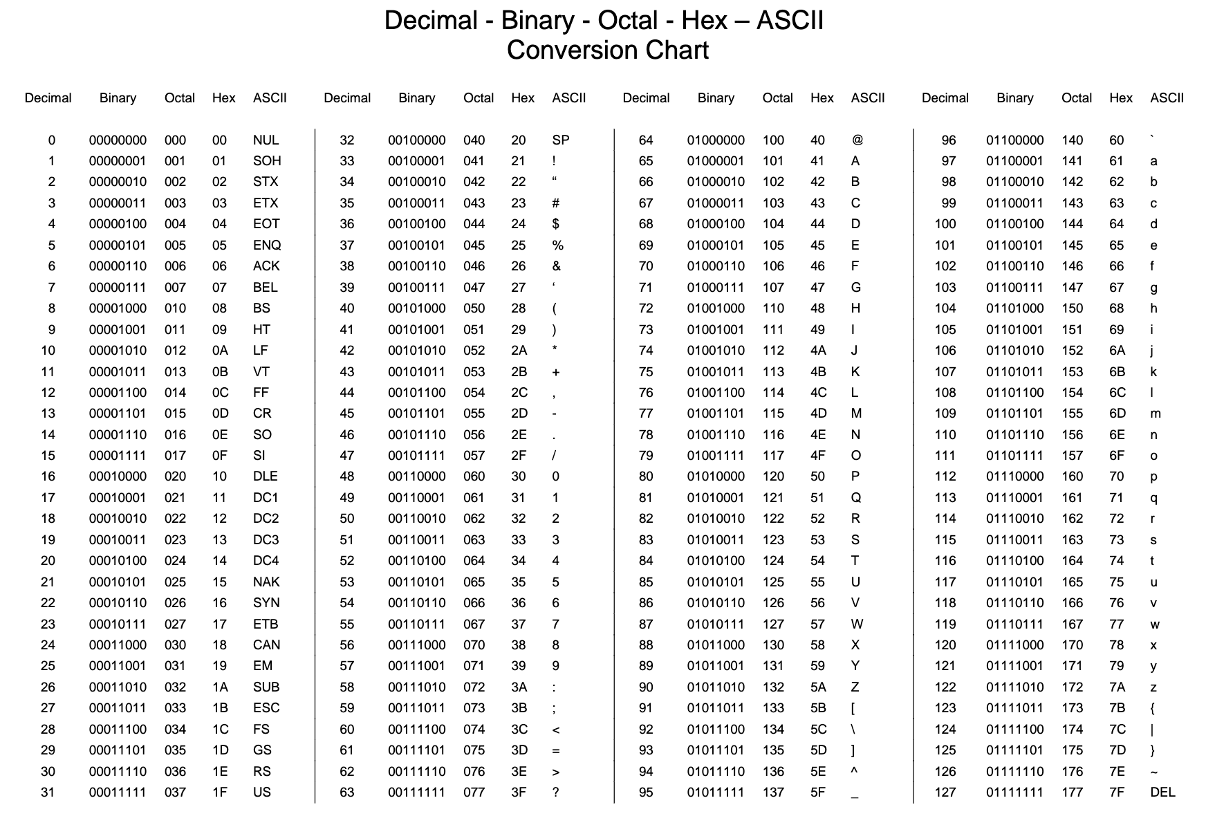
Part (4) of the (5) in Data Cleaning process! We are going to be working with different character encodings.
In computing, data storage, and data transmission, character encoding is used to represent a repertoire of characters by some kind of encoding system that assigns a number to each character for digital representation. Depending on the abstraction level and context, corresponding code points and the resulting code space may be regarded as bit patterns, octets, natural numbers, electrical pulses, etc. A character encoding is used in computation, data storage, and transmission of textual data. "Character set", "character map", "codeset" and "code page" are related, but not identical, terms.
In part (4) we will:
The first thing we will need to do is load in the libraries we will be using. Not our datasets, though: we will get to those later!
Important! Make sure we run this cell ourself or the rest of our code won't work!
# modules we will use
import pandas as pd
import numpy as np

# helpful character encoding module
import chardet

# set seed for reproducibility
np.random.seed(0)
Character encodings are specific sets of rules for mapping from raw binary byte strings (that look like this: 0110100001101001) to characters that make up human-readable text (like "hello world"). There are many different encodings, and if we tried to read in text with a different encoding that the one it was originally written in, we ended up with scrambled text called "mojibake" (said like mo-gee-bah-kay). Here is an example of mojibake:
æ–‡å—化ã??
we might also end up with a "unknown" characters. There are what gets printed when there is no mapping between a particular byte and a character in the encoding we are using to read our byte string in and they look like this:
����������
Character encoding mismatches are less common today than they used to be, but it is definitely still a problem. There are lots of different character encodings, but the main one we need to know is UTF-8.
UTF-8 is the standard text encoding. All Python code is in UTF-8 and, ideally, all our data should be as well. It is when things are not in UTF-8 that we run into trouble.
It was pretty hard to deal with encodings in Python 2, but thankfully in Python 3 it is a lot simpler. There are two main data types we will encounter when working with text in Python 3. One is is the string, which is what text is by default.
# start with a string
before = "This is the euro symbol: €"

# check to see what datatype it is
type(before)
str
The other data is the bytes data type, which is a sequence of integers. we can convert a string into bytes by specifying which encoding it is in:
# encode it to a different encoding, replacing characters that raise errors
after = before.encode("utf-8", errors = "replace")

# check the type
type(after)
bytes
If we look at a bytes object, we will see that it has a b in front of it, and then maybe some text after. That is because bytes are printed out as if they were characters encoded in ASCII. (ASCII is an older character encoding that does not really work for writing any language other than English.) Here we can see that our euro symbol has been replaced with some mojibake that looks like "\xe2\x82\xac" when it is printed as if it were an ASCII string.
# take a look at what the bytes look like
after
b'This is the euro symbol: \xe2\x82\xac'
When we convert our bytes back to a string with the correct encoding, we can see that our text is all there correctly, which is great! :)
# convert it back to utf-8
print(after.decode("utf-8"))
This is the euro symbol: €
However, when we try to use a different encoding to map our bytes into a string,, we get an error. This is because the encoding weare trying to use does not know what to do with the bytes we are trying to pass it. We need to tell Python the encoding that the byte string is actually supposed to be in.
We can think of different encodings as different ways of recording music. We can record the same music on a CD, cassette tape or 8-track. While the music may sound more-or-less the same, we need to use the right equipment to play the music from each recording format. The correct decoder is like a cassette player or a cd player. If we try to play a cassette in a CD player, it just won't work.
# try to decode our bytes with the ascii encoding
print(after.decode("ascii"))
---------------------------------------------------------------------------
UnicodeDecodeError                        Traceback (most recent call last)
<ipython-input-31-50fd8662e3ae> in <module>
      1 # try to decode our bytes with the ascii encoding
----> 2 print(after.decode("ascii"))

UnicodeDecodeError: 'ascii' codec can't decode byte 0xe2 in position 25: ordinal not in range(128)
We can also run into trouble if we try to use the wrong encoding to map from a string to bytes. As we mentioned, strings are UTF-8 by default in Python 3, so if we try to treat them like they were in another encoding we will create problems.
For example, if we try to convert a string to bytes for ascii using encode(), we can ask for the bytes to be what they would be if the text was in ASCII. Since our text is not in ASCII, though, there will be some characters it can not handle. We can automatically replace the characters that ASCII can not handle. If we do that, however, any characters not in ASCII will just be replaced with the unknown character. Then, when we convert the bytes back to a string, the character will be replaced with the unknown character. The dangerous part about this is that there is not way to tell which character it should have been. That means we may have just made our data unusable!
# start with a string
before = "This is the euro symbol: €"

# encode it to a different encoding, replacing characters that raise errors
after = before.encode("ascii", errors = "replace")

# convert it back to utf-8
print(after.decode("ascii"))

# We have lost the original underlying byte string! It is been
# replaced with the underlying byte string for the unknown character
This is the euro symbol: ?
This is not right and we want to avoid doing it! It is far better to convert all our text to UTF-8 as soon as we can and keep it in that encoding. The best time to convert non UTF-8 input into UTF-8 is when we read in files, which we will talk about next.
First, however, try converting between bytes and strings with different encodings and see what happens. Notice what this does to our text. Would we want this to happen to data we were trying to analyze?
Most files we will encounter will probably be encoded with UTF-8. This is what Python expects by default, so most of the time we won't run into problems. However, sometimes we will get an error like this:
# try to read in a file not in UTF-8
kickstarter_2016 = pd.read_csv("ks-projects-201612.csv")
Notice that we get the same UnicodeDecodeError we got when we tried to decode UTF-8 bytes as if they were ASCII! This tells us that this file is not actually UTF-8. We do not know what encoding it actually is though. One way to figure it out is to try and test a bunch of different character encodings and see if any of them work. A better way, though, is to use the chardet module to try and automatically guess what the right encoding is. It is not 100% guaranteed to be right, but it is usually faster than just trying to guess.
We are going to just look at the first ten thousand bytes of this file. This is usually enough for a good guess about what the encoding is and is much faster than trying to look at the whole file. (Especially with a large file this can be very slow.) Another reason to just look at the first part of the file is that we can see by looking at the error message that the first problem is the 11th character. So we probably only need to look at the first little bit of the file to figure out what is going on.
# look at the first ten thousand bytes to guess the character encoding
with open("ks-projects-201801.csv", 'rb') as rawdata:
    result = chardet.detect(rawdata.read(10000))

# check what the character encoding might be
print(result)
{'encoding': 'Windows-1252', 'confidence': 0.73, 'language': ''}
So chardet is 73% confidence that the right encoding is "Windows-1252". We will see if that is correct:
# read in the file with the encoding detected by chardet
kickstarter_2016 = pd.read_csv("ks-projects-201612.csv", encoding='Windows-1252')

# look at the first few lines
kickstarter_2016.head()
| ID | name | category | main_category | currency | deadline | goal | launched | pledged | state | backers | country | usd pledged | Unnamed: 13 | Unnamed: 14 | Unnamed: 15 | Unnamed: 16 | |
|---|---|---|---|---|---|---|---|---|---|---|---|---|---|---|---|---|---|
| 0 | 1000002330 | The Songs of Adelaide & Abullah | Poetry | Publishing | GBP | 2015-10-09 11:36:00 | 1000 | 2015-08-11 12:12:28 | 0 | failed | 0 | GB | 0 | NaN | NaN | NaN | NaN |
| 1 | 1000004038 | Where is Hank? | Narrative Film | Film & Video | USD | 2013-02-26 00:20:50 | 45000 | 2013-01-12 00:20:50 | 220 | failed | 3 | US | 220 | NaN | NaN | NaN | NaN |
| 2 | 1000007540 | ToshiCapital Rekordz Needs Help to Complete Album | Music | Music | USD | 2012-04-16 04:24:11 | 5000 | 2012-03-17 03:24:11 | 1 | failed | 1 | US | 1 | NaN | NaN | NaN | NaN |
| 3 | 1000011046 | Community Film Project: The Art of Neighborhoo... | Film & Video | Film & Video | USD | 2015-08-29 01:00:00 | 19500 | 2015-07-04 08:35:03 | 1283 | canceled | 14 | US | 1283 | NaN | NaN | NaN | NaN |
| 4 | 1000014025 | Monarch Espresso Bar | Restaurants | Food | USD | 2016-04-01 13:38:27 | 50000 | 2016-02-26 13:38:27 | 52375 | successful | 224 | US | 52375 | NaN | NaN | NaN | NaN |
Looks like chardet was right! The file reads in with no problem (although we do get a warning about datatypes) and when we look at the first few rows it seems to be be fine.
What if the encoding chardet guesses is not right? Since chardet is basically just a fancy guesser, sometimes it will guess the wrong encoding. One thing we can try is looking at more or less of the file and seeing if we get a different result and then try that.
Finally, once we have gone through all the trouble of getting our file into UTF-8, we will probably want to keep it that way. The easiest way to do that is to save our files with UTF-8 encoding. The good news is, since UTF-8 is the standard encoding in Python, when we save a file it will be saved as UTF-8 by default:
# save our file (will be saved as UTF-8 by default!)
kickstarter_2016.to_csv("ks-projects-201801-utf8.csv")
And we are completed!
If we have not saved a file in a kernel before, we need to hit the commit & run button and wait for our notebook to finish running first before we can see or access the file we have saved out. If we do not see it at first, wait a couple minutes and it should show up. The files we save will be in our work directory "../output/", and we can download them from our notebook.
Part (5) of the (5) in Data Cleaning process! We are going to be working with different character encodings.
Part (1) of the (5) in Data Cleaning process! we are going to learn how to clean up inconsistent text entries.
Typographic errors and spelling mistakes, can completely wreck even the most well-planned database. These types of errors are difficult to predict and often occur when data entry tasks are being performed by human beings. We simply get in a hurry and can get a little sloppy with our typing skills. Related to this is the common problem of having different entry styles among a variety of individuals. Different people might be in charge of putting data into the database. Some people like one abbreviation over another, and others will choose to spell out information completely. we will take a look at an example using the products table that we created in the last movie.
In part (5) we will:
The first thing we will need to do is load in the libraries we will be using.
Important! Make sure we run this cell ourself or the rest of our code won't work!
# modules we will use
import pandas as pd
import numpy as np

# helpful modules
import fuzzywuzzy
from fuzzywuzzy import process
import chardet

# set seed for reproducibility
np.random.seed(0)
When we tried to read in the PakistanSuicideAttacks Ver 11 (30-November-2017).csvfile the first time, we got a character encoding error, so we are going to quickly check out what the encoding should be...
# look at the first ten thousand bytes to guess the character encoding
with open("PakistanSuicideAttacks Ver 11 (30-November-2017).csv", 'rb') as rawdata:
    result = chardet.detect(rawdata.read(100000))

# check what the character encoding might be
print(result)
{'encoding': 'Windows-1252', 'confidence': 0.73, 'language': ''}
We will read it in with the correct encoding.
# read in our dat
suicide_attacks = pd.read_csv("PakistanSuicideAttacks Ver 11 (30-November-2017).csv",
                              encoding='Windows-1252')
Now we are ready to get started! We can, as always, take a moment here to look at the data and get familiar with it. :)
We will clean up the "City" column to make sure there is no data entry inconsistencies in it. We could go through and check each row by hand, of course, and hand-correct inconsistencies when we find them. There is a more efficient way to do this though!
# get all the unique values in the 'City' column
cities = suicide_attacks['City'].unique()

# sort them alphabetically and then take a closer look
cities.sort()
cities
array(['ATTOCK', 'Attock ', 'Bajaur Agency', 'Bannu', 'Bhakkar ', 'Buner',
       'Chakwal ', 'Chaman', 'Charsadda', 'Charsadda ', 'D. I Khan',
       'D.G Khan', 'D.G Khan ', 'D.I Khan', 'D.I Khan ', 'Dara Adam Khel',
       'Dara Adam khel', 'Fateh Jang', 'Ghallanai, Mohmand Agency ',
       'Gujrat', 'Hangu', 'Haripur', 'Hayatabad', 'Islamabad',
       'Islamabad ', 'Jacobabad', 'KURRAM AGENCY', 'Karachi', 'Karachi ',
       'Karak', 'Khanewal', 'Khuzdar', 'Khyber Agency', 'Khyber Agency ',
       'Kohat', 'Kohat ', 'Kuram Agency ', 'Lahore', 'Lahore ',
       'Lakki Marwat', 'Lakki marwat', 'Lasbela', 'Lower Dir', 'MULTAN',
       'Malakand ', 'Mansehra', 'Mardan', 'Mohmand Agency',
       'Mohmand Agency ', 'Mohmand agency', 'Mosal Kor, Mohmand Agency',
       'Multan', 'Muzaffarabad', 'North Waziristan', 'North waziristan',
       'Nowshehra', 'Orakzai Agency', 'Peshawar', 'Peshawar ', 'Pishin',
       'Poonch', 'Quetta', 'Quetta ', 'Rawalpindi', 'Sargodha',
       'Sehwan town', 'Shabqadar-Charsadda', 'Shangla ', 'Shikarpur',
       'Sialkot', 'South Waziristan', 'South waziristan', 'Sudhanoti',
       'Sukkur', 'Swabi ', 'Swat', 'Swat ', 'Taftan',
       'Tangi, Charsadda District', 'Tank', 'Tank ', 'Taunsa',
       'Tirah Valley', 'Totalai', 'Upper Dir', 'Wagah', 'Zhob', 'bannu',
       'karachi', 'karachi ', 'lakki marwat', 'peshawar', 'swat'],
      dtype=object)
We can see some problems due to inconsistent data entry: 'Lahore' and 'Lahore ', for example, or 'Lakki Marwat' and 'Lakki marwat'.
The first thing we are going to do is make everything lower case (we can change it back at the end if we like) and remove any white spaces at the beginning and end of cells. Inconsistencies in capitalizations and trailing white spaces are very common in text data and we can fix a good 80% of our text data entry inconsistencies by doing this.
# convert to lower case
suicide_attacks['City'] = suicide_attacks['City'].str.lower()
# remove trailing white spaces
suicide_attacks['City'] = suicide_attacks['City'].str.strip()
Next we are going to tackle more difficult inconsistencies.
We will look at the city column and see if there is any more data cleaning we need to do.
# get all the unique values in the 'City' column
cities = suicide_attacks['City'].unique()

# sort them alphabetically and then take a closer look
cities.sort()
cities
array(['attock', 'bajaur agency', 'bannu', 'bhakkar', 'buner', 'chakwal',
       'chaman', 'charsadda', 'd. i khan', 'd.g khan', 'd.i khan',
       'dara adam khel', 'fateh jang', 'ghallanai, mohmand agency',
       'gujrat', 'hangu', 'haripur', 'hayatabad', 'islamabad',
       'jacobabad', 'karachi', 'karak', 'khanewal', 'khuzdar',
       'khyber agency', 'kohat', 'kuram agency', 'kurram agency',
       'lahore', 'lakki marwat', 'lasbela', 'lower dir', 'malakand',
       'mansehra', 'mardan', 'mohmand agency',
       'mosal kor, mohmand agency', 'multan', 'muzaffarabad',
       'north waziristan', 'nowshehra', 'orakzai agency', 'peshawar',
       'pishin', 'poonch', 'quetta', 'rawalpindi', 'sargodha',
       'sehwan town', 'shabqadar-charsadda', 'shangla', 'shikarpur',
       'sialkot', 'south waziristan', 'sudhanoti', 'sukkur', 'swabi',
       'swat', 'taftan', 'tangi, charsadda district', 'tank', 'taunsa',
       'tirah valley', 'totalai', 'upper dir', 'wagah', 'zhob'],
      dtype=object)
It does look like there are some remaining inconsistencies: 'd. i khan' and 'd.i khan' should probably be the same. (We looked it up and 'd.g khan' is a seperate city, so we should not combine those.)
We are going to use the fuzzywuzzy package to help identify which string are closest to each other. This dataset is small enough that we could probably could correct errors by hand, but that approach does not scale well. It is challenge to correct thousand of data! Automating things as early as possible is generally a good idea.
Fuzzy matching: The process of automatically finding text strings that are very similar to the target string. In general, a string is considered "closer" to another one the fewer characters we would need to change if we were transforming one string into another. So "apple" and "snapple" are two changes away from each other (add "s" and "n") while "in" and "on" and one change away (rplace "i" with "o"). We won't always be able to rely on fuzzy matching 100%, but it will usually end up saving us at least a little time.
Fuzzywuzzy returns a ratio given two strings. The closer the ratio is to 100, the smaller the edit distance between the two strings. We are going to get the ten strings from our list of cities that have the closest distance to "d.i khan".
# get the top 10 closest matches to "d.i khan"
matches = fuzzywuzzy.process.extract("d.i khan", cities, limit=10, scorer=fuzzywuzzy.fuzz.token_sort_ratio)

# take a look at them
matches
[('d. i khan', 100),
 ('d.i khan', 100),
 ('d.g khan', 88),
 ('khanewal', 50),
 ('sudhanoti', 47),
 ('hangu', 46),
 ('kohat', 46),
 ('dara adam khel', 45),
 ('chaman', 43),
 ('mardan', 43)]
We can see that two of the items in the cities are very close to "d.i khan": "d. i khan" and "d.i khan". We can also see the "d.g khan", which is a seperate city, has a ratio of 88. Since we do not want to replace "d.g khan" with "d.i khan", we will replace all rows in our City column that have a ratio of > 90 with "d. i khan".
We are going to write a function. It is a good idea to write a general purpose function we can reuse if we think we might have to do a specific task more than once or twice. This keeps us from having to copy and paste code too often, which saves time and can help prevent mistakes.
# function to replace rows in the provided column of the provided dataframe
# that match the provided string above the provided ratio with the provided string
def replace_matches_in_column(df, column, string_to_match, min_ratio = 90):
    # get a list of unique strings
    strings = df[column].unique()

    # get the top 10 closest matches to our input string
    matches = fuzzywuzzy.process.extract(string_to_match, strings,
                                         limit=10, scorer=fuzzywuzzy.fuzz.token_sort_ratio)

    # only get matches with a ratio > 90
    close_matches = [matches[0] for matches in matches if matches[1] >= min_ratio]

    # get the rows of all the close matches in our dataframe
    rows_with_matches = df[column].isin(close_matches)

    # replace all rows with close matches with the input matches
    df.loc[rows_with_matches, column] = string_to_match

    # let us know the function's done
    print("All done!")
Now that we have a function, we can put it to the test!
# use the function we just wrote to replace close matches to "d.i khan" with "d.i khan"
replace_matches_in_column(df=suicide_attacks, column='City', string_to_match="d.i khan")
All done!
We will check the unique values in our City column again and make sure we have tidied up d.i khan correctly.
# get all the unique values in the 'City' column
cities = suicide_attacks['City'].unique()

# sort them alphabetically and then take a closer look
cities.sort()
cities
array(['attock', 'bajaur agency', 'bannu', 'bhakkar', 'buner', 'chakwal',
       'chaman', 'charsadda', 'd.g khan', 'd.i khan', 'dara adam khel',
       'fateh jang', 'ghallanai, mohmand agency', 'gujrat', 'hangu',
       'haripur', 'hayatabad', 'islamabad', 'jacobabad', 'karachi',
       'karak', 'khanewal', 'khuzdar', 'khyber agency', 'kohat',
       'kuram agency', 'kurram agency', 'lahore', 'lakki marwat',
       'lasbela', 'lower dir', 'malakand', 'mansehra', 'mardan',
       'mohmand agency', 'mosal kor, mohmand agency', 'multan',
       'muzaffarabad', 'north waziristan', 'nowshehra', 'orakzai agency',
       'peshawar', 'pishin', 'poonch', 'quetta', 'rawalpindi', 'sargodha',
       'sehwan town', 'shabqadar-charsadda', 'shangla', 'shikarpur',
       'sialkot', 'south waziristan', 'sudhanoti', 'sukkur', 'swabi',
       'swat', 'taftan', 'tangi, charsadda district', 'tank', 'taunsa',
       'tirah valley', 'totalai', 'upper dir', 'wagah', 'zhob'],
      dtype=object)
We only have "d.i khan" in our dataframe and we did not have to change anything by hand.